Hypothesis Testing // Statistics Basics
Data Science Assignment #5

Welcome, everyone, to our statistics beginnings! When I started this unit, I hadn’t done any statistics since my freshman year of college, so it had been quite a few years. Luckily, we will start off slow and work our way up. Understanding these basics will be very important as we move forward. Also, statistics questions often come up in data science interviews, so it’s good to remember how to set up hypothesis tests, what a null hypothesis is, and what a p value of .05 actually means. We’ll be going over all of these today! Let’s do it!
We’ll start with some statistics basics:
A hypothesis is a claim about some aspect of a population. A hypothesis test allows us to test the claim about the population and find out how likely it is to be true. The hypothesis test consists of several components; two statements, the null hypothesis and the alternative hypothesis, the test statistic and the critical value, which in turn give us the P-value and the rejection region (𝛼), respectively.
The null hypothesis, denoted as 𝐻0 is the statement that the value of the parameter is, in fact, equal to the claimed value. We assume that the null hypothesis is true until we prove that it is not. In statistical answers, we generally “fail to reject the null hypothesis”, if we think that it is true.
The alternative hypothesis, denoted as 𝐻1 is the statement that the value of the parameter differs in some way from the null hypothesis. The alternative hypothesis can use the symbols <, >, 𝑜𝑟 ≠. We never “accept the alternative hypothesis”, rather, we “reject the null hypothesis”.
The test statistic is the tool we use to decide whether or not to reject the null hypothesis. It is obtained by taking the observed value (the sample statistic) and converting it into a standard score under the assumption that the null hypothesis is true.
The P-value for any given hypothesis test is the probability of getting a sample statistic at least as extreme as the observed value. That is to say, it is the area to the left or right of the test statistic. A p-value is the probability that the results from the data occurred by chance. P-values range from 0 to 100%, and are written as decimals. Low p-values are good, indicating the data did not result by chance.
The critical value is the standard score that separates the rejection region (𝛼) from the rest of a given curve.
A t-test is a statistical test that compares the averages of two samples. Basically, the goal is to determine if the results could have happened by chance, or if the results are statistically significant (this is the only term I remembered from my college stats class). The null hypothesis is that the difference in group means is zero, and the alternate hypothesis is that the difference in group means is not zero.
The t score is a ratio between the difference between two groups and the difference within the groups. A large t-score tells you that the groups are different. A small t-score tells you that the groups are similar.
Types of Errors:
Type I Error: incorrectly rejecting a true null hypothesis (false negative)
Type II Error: incorrectly failing to reject an untrue null hypothesis (false positive).

https://www.google.com/url?sa=i&url=https%3A%2F%2Fwww.youtube.com%2Fwatch%3Fv%3DDlwOTOydeyk&psig=AOvVaw0hHgkDYGkKJZhBc8jh71f7&ust=1631932889589000&source=images&cd=vfe&ved=0CAsQjRxqFwoTCNi2-fP9hPMCFQAAAAAdAAAAABAJ
I recommend checking out this site for some additional info, if you need more review!
Now to our assignment. Here is the background for our data and task:
The Mosquito.xlsx dataset contains data recorded in an experiment conducted on male soldiers in the Indian Army who were stationed in the Tezpur/Solmara garrison in Northeast India. Thirty soldiers were randomly selected to receive one of three types of mosquito single repellent patch. After giving informed consent, the study participants affixed the patches at predetermined points on their uniforms and research assistants (who were blinded to the type of repellent used) counted the number of times a mosquito landed on each individual in an hour.
Medical officers with the Indian Army have recorded data on mosquito bites and related illness for many years and can say with authority that the mean number of mosquito touches for soldiers not wearing any mosquito repellent is 8.2 per hour. We wish to determine if wearing a single repellent patch changes the mean number of mosquito touches for soldiers compared to not wearing any mosquito repellant.
Adapted from: A. Bhatnagar and V.K. Mehta (2007). "Efficacy of Deltamethrin and Cyfluthrin Impregnated Cloth Over Uniform Against Mosquito Bites," Medical Journal Armed Forces India, Vol. 63, pp. 120-122.
For task one, we will load in our data and save it to a DataFrame names df_mosquito. Also, we’ll load in pandas and numpy like always.
# Task 1

import pandas as pd
import numpy as np

# URL for the dataset
data_url = 'https://raw.githubusercontent.com/LambdaSchool/data-science-practice-datasets/main/unit_1/Mosquito/Mosquito.csv'

# Save the DF
df_mosquito = pd.read_csv(data_url)

# Print DataFrame head
df_mosquito.head()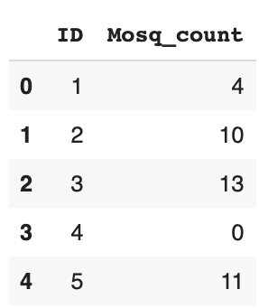
Task two asks us to state our null and alternative hypotheses for the experiment.
𝐻0: 𝜇= 8.2
𝐻𝑎: 𝜇≠ 8.2
In task three we will calculate the mean number of mosquito touches in the sample. Then, we’ll save the value to a variable named mosquito_touch_mean.
# Task 3

# Use .describe() to view stats info
print(df_mosquito.describe())

# Save the mean value
mosquito_touch_mean = 8.01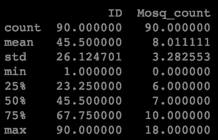
Now for task four, we’ll calculate the standard deviation. Numpy has a very useful function for this: .std()! And that’s it! We’ll save this value to a variable as well.
# Task 4

# View standard deviation info
print(df_mosquito.std())

# Save mosquito touch STD
mosquito_touch_std = 3.28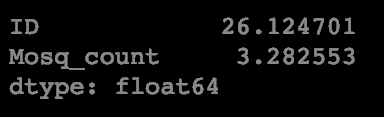
Task five asks us to conduct a 1-sample t-test to test our hypotheses. We’ll need to import the stats package from scipy to get this information. The stats.ttest_1sam() function returns two values: the p value is the second value that it returns. This is the value we need to evaluate our t-test, so we’ll save this value to a variable.
# Task 5

# Import stats
from scipy import stats

# Use stats.ttest_1sam() function to save p value
stat, mosquito_pval = stats.ttest_1samp(df_mosquito['Mosq_count'], popmean=8.2)

print(mosquito_pval)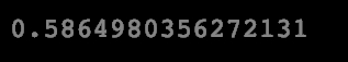
In task six, we are asked to report our conclusion at the 0.05 significance level. My simple answer would be as follows: We fail to reject the null hypthesis, because the p value was 0.59, which is greater than the .05 significance level. So, those using the repellent patches didn't have a statistically significant difference in interactions with mosquitos.
The rest of the assignment brings us to different data and another hypothesis test!
More than 14,000 people finished the 2020 Disney Marathon held on January 12. The results by age and gender group are included in the Disney.csv dataset.
We wish to determine if the mean finishing time for male and female marathon runners is the same or if there is a difference in the mean finishing time between male and female marathon runners.
Source: Track Shack. 2020 Disney Marathon Race Results
Since we have a new dataset, task seven asks us to load in the new data. We’ll save this one as df_disney.
# Task 7

# URL for Disney marathon dataset
data_url2 = 'https://raw.githubusercontent.com/LambdaSchool/data-science-practice-datasets/main/unit_1/Disney_Marathon/Disney.csv'

# Save the DataFrame
df_disney = pd.read_csv(data_url2, index_col=None)

df_disney.head()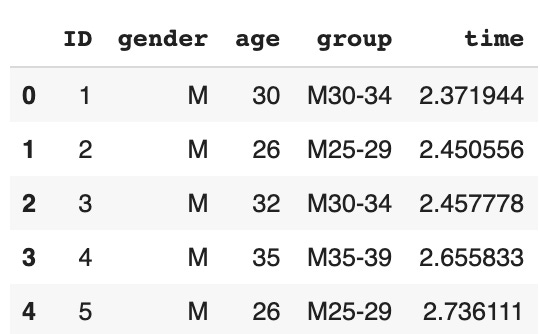
For task eight, we’ll write our new null and alternative hypotheses:
𝐻0: 𝜇 = female time mean = male time mean
𝐻𝑎: 𝜇 ≠ female time mean = male time mean
In task nine, we’ll create two new series from our DataFrame: one containing finishing times for male participants and one for female participants. I used a .loc statement, based on the value of the gender column in the DataFrame, to create separate DataFrames for male and females. Then, a series is as simple as selecting what column you want from the DataFrame.
# Task 9

# Create new DataFrames based on gender
male_finishing = df_disney.loc[df_disney['gender'] == 'M']
female_finishing = df_disney.loc[df_disney['gender'] == 'F']

# Create a series for male times and female times
male_finish = male_finishing['time']
female_finish = female_finishing['time']

print(male_finish.head())
print(female_finish.head())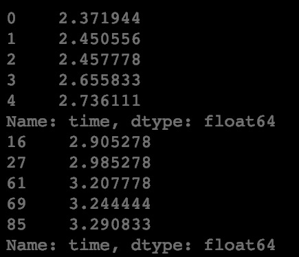
For task ten, we’ll calculate the mean finishing times for males and females.
# Task 10

# Find the mean times
male_finish_mean = male_finish.mean()
female_finish_mean = female_finish.mean()

# Print the values
print(male_finish_mean)
print(female_finish_mean)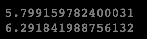
For task eleven, we’ll calculate the standard deviation of male and female finishing times.
# Task 11

# Find the standard deviations
male_finish_std = male_finish.std()
female_finish_std = female_finish.std()

# Print the values
print(male_finish_std)
print(female_finish_std)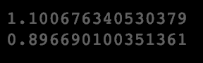
Now, for task twelve we’ll conduct a 2-sample t-test to test our hypotheses. We’ll save both our t-statistic and p-values to variables, the results from using the stats.ttest_ind() function.
# Task 12

# Use stats.ttest_ind() function to get info
disney_tval, disney_pval = stats.ttest_ind(male_finish, female_finish)

print(disney_tval)
print(disney_pval)
Task thirteen asks us to report our conclusion at the 0.05 significance level. Here is my answer: The p value of the test was less than 0.05, so we reject the null hypotheses and conclude that the difference in men and women's mean race times were statistically significant.
Task 14 asks us to explain the Central Limit Theorem: When more independent variables are added, their normalized sum tends toward a normal distribution.
Task 15 asks us to describe the Normal Distribution: The probability distribution that naturally occurs in many instances, bell shaped; normally it's expected. (mean=median=mode)
Task 16 asks us to describe the relationship between the Normal distribution and the t-distribution: The t-distribution is the probability distribution of a sample, and as the sample size grows, the distribution becomes more similar to the normal distribution.
Task 17 asks us to write about who William Sealy Gosset was: Gosset developed the t-test and t-distribution under the pseudonym "Student". Also, he was the head brewer of Guiness. A cool guy.
There you have it: the first statistics assignment of the data science course. A little info on hypothesis tests, distributions, and more. I hope this helped to learn a little bit about statistics basics, and we’ll keep going from here next week! Let me know if you have any questions working through the material!
XOXO,
Ash